The .flac format: linear predictive coding and rice codes
01 Apr 2018Introduction
FLAC stands for Free Lossless Audio Codec and it’s the standard open source codec used for lossless audio compression. In this post I would like to use the .flac example to explore how lossless audio compression is possible and focus on the two core aspects of it: linear predictive coding and entropy coding with Rice codes.
TL;DR
Most lossless audio compression codecs work very similarly: they split the audio stream in multiple blocks or frames and then compress each one of them. Compression is achieved identifying and modelling the structure in the audio signal: any repeating pattern is redundant by definition and can instead be represented more efficiently using a mathematical model and its parameters. These models need not to be complicated: constant values can already model silence blocks while linear predictive coding (a linear autoregressive model) is used for the other blocks. In order to recreate the signal without loss the approximation residuals of the models are also saved, but using a coding scheme optimised for their distribution. Linear predictive coding leads to residual Laplace-distributed and hence usually the Rice coding scheme is used.
Linear predictive coding
Linear predictive coding is a modelling technique equivalent to an \(AR(p)\) auto regressive model: the signal \(X_t\) at time \(t\) is modelled as a linear combination of its previous \(p\) values.
More formally, let \({X_t}\) be a wide sense stationary (WSS) stochastic process with zero mean, which is:
\[ \begin{equation}\label{eqn:wss_1} E[X_t] = \mu = 0 \quad \forall t \end{equation} \]
\[
\begin{equation}\label{eqn:wss_2}
Cov[X_{t}, X_{t + \tau}] = Cov[X_{t+h}, X_{t +h + \tau}] \quad \forall t \ \forall h
\end{equation}
\]
From \ref{eqn:wss_1} and \ref{eqn:wss_2} it follows that the covariance function only depends on the lag \(\tau\) and can be expressed in terms of the autocorrelation function \(R(\tau)\):
\[ \begin{equation}\label{eqn:autocorr} Cov[X_{t}, X_{t + \tau}] = E[(X_t - \mu)(X_{t + \tau} - \mu)] = E[X_tX_{t+\tau}] = R(\tau) \end{equation} \]
where \(R(\tau) = R(-\tau)\) is symmetric.
Now assume that we wanted to approximate each value \(X_t\) as a linear combination of its previous \(p\) values:
\[ \hat{X_t} = \sum_{k = 1}^{p}\alpha_k X_{t-k} \]
let \(\boldsymbol{\boldsymbol{\alpha}} = \begin{bmatrix} \alpha_1 & \cdots & \alpha_p \end{bmatrix}^\top \), then the approximation error \(\epsilon_t\) at time t is the random variable:
\[ \epsilon_t = X_t - \hat{X_t} = X_t - \mathbf{\boldsymbol{\alpha}}^\top \begin{bmatrix} X_{t-1} \\ \vdots \\ X_{t-p} \end{bmatrix} = X_t - \mathbf{\boldsymbol{\alpha}}^\top \mathbf{X_{t-1:t-p}} \]
For an optimal approximation we then chose \(\boldsymbol{\alpha}\) so that it minimises the expected squared estimation error. To derive the solution we make use of the orthogonality principle.
Lemma: Orthogonality principle.
The estimate \(\hat{X_t} \) minimises the expected squared error if and only if the estimation error \(\epsilon_t\) is orthogonal to the \(p\) random variables \(X_{t-1}, …, X_{t-p}\), ie if and only if: \[ E[\epsilon_t X_{t-i}] = 0 \quad \forall 1 \leq i \leq p \]
From the orthogonality principle we can derive the Yule-Walker equations:
\[ \begin{equation} \begin{split} \mathbf{0} = & E[\epsilon_t \mathbf{X_{t-1:t-p}}] \\ = & E[(X_t - \mathbf{X_{t-1:t-p}}^\top\alpha)\mathbf{X_{t-1:t-p}}] \\ = & E[X_t \mathbf{X_{t-1:t-p}} - \mathbf{X_{t-1:t-p}}^\top\boldsymbol{\alpha}\mathbf{X_{t-1:t-p}}] \\ = & E[X_t \mathbf{X_{t-1:t-p}} - trace(\mathbf{X_{t-1:t-p}}^\top\boldsymbol{\alpha}\mathbf{X_{t-1:t-p}})] \\ = & E[X_t \mathbf{X_{t-1:t-p}} - trace(\mathbf{X_{t-1:t-p}}\mathbf{X_{t-1:t-p}}^\top\boldsymbol{\alpha})] \\ = & E[X_t \mathbf{X_{t-1:t-p}} - \mathbf{X_{t-1:t-p}}\mathbf{X_{t-1:t-p}}^\top\boldsymbol{\alpha}] \\ = & E[X_t \mathbf{X_{t-1:t-p}}] - E[ \mathbf{X_{t-1:t-p}}\mathbf{X_{t-1:t-p}}^\top]\boldsymbol{\alpha} \\ \end{split} \end{equation}\label{eqn:yw1} \]
Using \ref{eqn:autocorr} we can rewrite \( E[ \mathbf{X_{t-1:t-p}}\mathbf{X_{t-1:t-p}}]^\top = \mathbf{R}\) as:
\[ \mathbf{R} = \begin{bmatrix} R(0) & R(1) & R(2) & \cdots & R(p-1) \\ R(1) & R(0) & R(1) & \cdots & R(p-2) \\ R(2) & R(1) & R(0) & \cdots & R(p-3) \\ \vdots & \vdots & \vdots & & \vdots \\ R(p-1) & R(p-2) & R(p-3) & \cdots & R(0) \\ \end{bmatrix} \]
and by defining \(\mathbf{r} = \begin{bmatrix} R(1) & \cdots & R(p) \end{bmatrix}^\top\) we can finally rewrite \ref{eqn:yw1} as:
\begin{equation}\label{eqn:yh2}
\mathbf{R}\boldsymbol{\alpha} = \mathbf{r}
\end{equation}
In this form we can solve for \(\boldsymbol{\alpha}\) given estimates of \(\mathbf{R}\) and \(\mathbf{r}\)
The matrix \(\mathbf{R}\) is a toeplitz matrix. A toeplitz matrix has the property that each descending diagonal from left to right is constant and for these matrices there is an algorithm, the Levinson–Durbin recursion, that can solve the system in \(O(p^2)\) which is much better than simply inverting \(\mathbf{R}\), which would have a cost \(O(p^3)\). The overall computational cost is thus \(O(np + p^2)\) where the first term comes from the cost of computing the sample estimate of the auto correlation matrix.
Comparison with ordinary least squares
The previous model could have been expressed as an instance of a general linear regression model whose covariates are the \(p\) lagged values. The solution would then minimise for the expected mean squared error directly without making assumptions about the underlying WSS property. This leads to a very similar but more expensive solution, as we lose the benefit of the WSS assumption.
The normal equations for the general linear regression problem are: \[ (\mathbf{X}^\top \mathbf{X})\mathbf{\boldsymbol{\alpha}} = \mathbf{X}^\top \mathbf{y} \]
where: \[ \mathbf{y} = \begin{bmatrix} y_{p+1}\\ \vdots \\ y_n \\ \vdots \\ y_N \end{bmatrix} \]
\[
\mathbf{X} = \begin{bmatrix}
y_p & y_{p-1} & \cdots & y_0 \\
\vdots &\vdots & &\vdots \\
y_n & y_{n-1} & \cdots & y_{n-p} \\
\vdots &\vdots & &\vdots \\
y_N & y_{N-1} & \cdots & y_{N-p} \\
\end{bmatrix}
\]
\[ \mathbf{\boldsymbol{\alpha}} = \begin{bmatrix} \alpha_1\\ \vdots \\ \alpha_p \\ \end{bmatrix} \]
It is easy to notice the similarities with equation \ref{eqn:yh2} : this solution is computing the sample estimates of \(\mathbf{R}\) and \( \mathbf{r}\), but using a different subset of samples for each estimate. Because of this the estimates have to be recomputed for each entry, and the toeplitz structure is lost, rsulting in higher estimation costs to build the matrices and higher matrix inversion costs to solve for \(\boldsymbol{\alpha}\). The computational complexity of this solution is \(O(n^2p + p^3)\), where the first term comes from the inner product of the matrix of covariates and the second term from its inversion. Usually \(n \gg p\) and thus this solution has complexity \(O(n^2p)\) which is much worst than the previous result of \(O(np)\) when using \ref{eqn:yh2}!
Entropy coding and Rice codes
Suppose one was to observe a realisation of the above mentioned stochastic process, for example an audio signal, and used LPC or some other model to approximate it. In order to reconstruct the original signal without any approximation error it is necessary to know what the exact realisation of the these error were and add them back into the reconstruction. The problem of efficiently storing these residuals is an instance of entropy coding.
Let’s start by defining what a code is. Assume the observed data can be modelled as a discrete random variable (note that we redefine (X) from the previous section): \[ X : \Omega \rightarrow \boldsymbol{\chi} \] where \(P(x \in X) = P(x)\)
now, given an alphabet of symbols \(\Sigma\), in the digital case \(\Sigma = \{0, 1\}\), a code is defined as
\[ C : \boldsymbol{\chi} \rightarrow \Sigma^* \]
\(C(x)\) is the code associated with \(x\), \(l(C(x))\) its length and therefore the expected length of a code is: \[l(C) = E_{x \sim P(x)}[l(C(x))] = \sum_{x \in \chi} P(x)l(C(x))\]
when designing or choosing a code the objective is to minimise \(l(C)\) for the distribution of input words \(p(x)\), so that the encoded input will require on average the least number of symbols. This is the problem referred to as entropy coding
A good general code that works for any input distribution is the Huffman code [1], and is for example used in the popular compression tool gzip. When the distribution of the input is known a priori though it is possible to use a coding scheme tailored for that distribution.
For example for the case of reconstruction errors the occurrence of small values in the input stream is significantly more likely than large values, which makes having smaller code words that cannot be confused to be the prefix of longer code words very convenient to encode them. A code in which no code-word is allowed to be the prefix of another code-word is called a prefix code and for the case of alphabets following a geometric distribution it can be shown that the optimal prefix code is the Golomb code [2].
Golomb coding [3] was invented by Solomon W. Golomb in the 1960s. It takes the input \(s\) and divides it by the tunable parameter \(m\). First the quotient is encoded in unary coding and then the remainder is econded in truncated binary coding. Rice coding is a special case of Golomb coding where \(m = 2^k\), which is faster to encode and decode thanks to the usage of powers of 2. It is very intuitive to understand how the coding scheme works just by looking at the follwowing table example
| Golomb | m=1 | m=2 | m=3 | m=4 | m=5 | m=6 | m=7 | m=8 |
|---|---|---|---|---|---|---|---|---|
| Rice | k=0 | k=1 | k=2 | k=3 | ||||
| s = 0 | 0 | 00 | 00 | 000 | 000 | 000 | 000 | 0000 |
| 1 | 10 | 01 | 010 | 001 | 001 | 001 | 0010 | 0001 |
| 2 | 110 | 100 | 011 | 010 | 010 | 0100 | 0011 | 0010 |
| 3 | 1110 | 101 | 100 | 011 | 0110 | 0101 | 0100 | 0011 |
| 4 | 11110 | 1100 | 1010 | 1000 | 0111 | 0110 | 0101 | 0100 |
| 5 | \(1^50\) | 1101 | 1011 | 1001 | 1000 | 0111 | 0110 | 0101 |
| 6 | \(1^60\) | 11100 | 1100 | 11010 | 1001 | 1000 | 0111 | 0110 |
| 7 | \(1^70\) | 11101 | 11010 | 1011 | 1010 | 1001 | 1000 | 0111 |
| 8 | \(1^80\) | 111100 | 11100 | 11000 | 10110 | 10100 | 10010 | 1000 |
| … | … | … | … | … | … | … | … | … |
The FLAC codec
Now we can see how modelling and entropy coding can be combined to form a lossless audio codec, bet let’s first start with an overview of how the strem is structured.
FLAC is mainly based on shorten [4], with additional features for more convenient use in real case consumer scenarios. A high level overview of the codec can be found here, while the definition of the stream is defined more precisly here
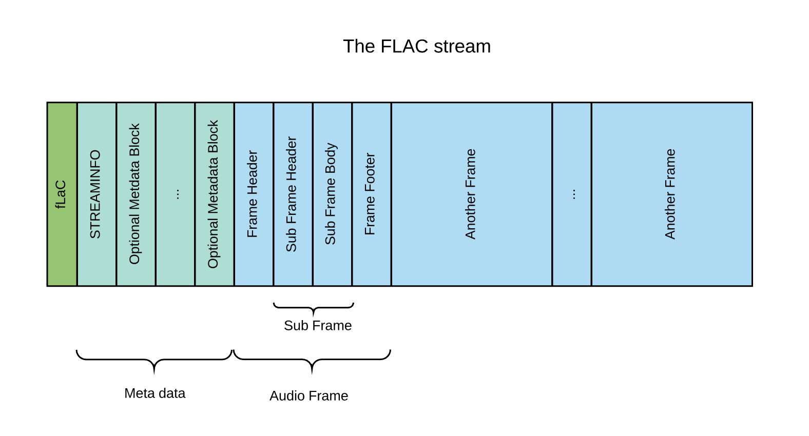
The basic structure of a FLAC stream is:
- the four byte string “fLaC” to identify the stream
- the STREAMINFO metadata block
- zero or more other metadata blocks
- one of more audio frames
FLAC defines various metadata blocks. They can be used for padding, seek tables, tags, cue sheets, and even application-specific data. There is no metadata block for the ID3 tags (where the artist, album, etc info are usually stored) but the world doesn’t really care and most decoders, including the reference one, know how to handle them anyway.
The only mandatory block is the STREAMINFO block. This block contains information like the sample rate, number of channels, etc., and additional data that can help the decoder manage its buffers like the minimum and maximum data rate and minimum and maximum block size. Also included in the STREAMINFO block is the MD5 signature of the unencoded audio data, useful for checking an entire stream for transmission errors.
Following the metadata blocks there is the sequence of frames containing the compressed audio stream: FLAC first splits the un-encoded audio data into blocks and then encodes each block separately. The blocking procedure serves two purposes: it is possible to un-compress, edit and re-compress only a subset of the frames at a time and it allows for the compression parameters to change over time, which is ideal since the audio signal is most certainly not stationary (but can be approximated as such within each block). The encoded data block is then packed into a frame with a header and a footer, and is appended to the stream. There is a trade-off in choosing the block size: smaller blocks allow for better compression but require more frame headers / footers to be stored. The reference implementation defaults to a block-size of 4096 samples, which at a sampling rate of 44.1kHz equals about 93 milliseconds but in theory blocks could be of variable length.
Compressing the audio signal in each data block
The raw encoding of an audio signal is extremely space inefficient: your common 16 bit 44.1kHz raw audio signal is encoded by storing each second of audio signal as a sequence of 44100 16 bit numbers (that is 88 KB/s!) representing the quantised discrete values of the audio wave over time. Any structure in the audio signal is just encoded as it comes: any moment of silence takes as much space as the most explosive of the cymbals!
At a high level, the compression procedure reduces the redundancy in the raw representation by identifying and modelling structured patterns in the raw signal: it exploits this patterns to approximate the raw signal using a mathematical function, and then stores the approximation errors so that it can revert them and recreate the original signal with no loss of information. Compression is achieved because storing both parts is much more efficient than storing the original raw signal: the approximated signal is saved by storing the parameters of its mathematical model and the approximation errors are also saved more efficiently because their distribution can be assumed a priori, and based on that an appropriate coding scheme is chosen.
More specifically the model being fitted to the signal by FLAC can either be a constant value (for silent moments), LPC or a fixed polynomial predictor from a subset of 4 that usually work well. Fixed polynomial prediction is much faster do decode and takes less space to store, as it has no parameters, but is less accurate than LPC. The higher the maximum LPC order \(p\), the slower but more accurate the model will be, but there are diminishing returns with increasing orders: \(p = 1\) already leads to good compression, while higher orders increase the required computation time with smaller compression benefits. The approximation error is then obtained by subtracting the original signal with the approximated signal. Empirically they are Laplace distributed, and can be assumed to be uncorrelated, so they can efficiently be encoded independently using Rice coding scheme (taking into account the presence of the sign bit).
These procedure is applied to both channel, left and right independently but a neat trick that can be used to often increase the compression of the block is to switch from left-right to mid-side (mid = (left + right) / 2, side = left - right).
After the modelling choice, the block is then encoded. First a sub frame is built, marking the model used in the header and encoding the audio content in the sub frame body. For example, in the case of LPC the sub frame body contains the \(p\) initial samples, the LPC coefficient and then the sequence of the encoded residuals. Finally the frame is constructed by preceding the sub frame with a frame header ant trailing it with a frame footer. The header starts with a sync code, and contains the minimum information necessary for a decoder to play the stream, like sample rate, bits per sample, etc. It also contains the block or sample number and an 8-bit CRC of the frame header. The frame footer contains a 16-bit CRC of the entire encoded frame for error detection. If the reference decoder detects a CRC error it will generate a silent block.
Bibliography
[1] David A Huffman. “A method for the construction of minimum-redundancy codes”. In: Proceedings of the IRE 40.9 (1952), pp. 1098–1101.
[2] Robert Gallager and David Van Voorhis. “Optimal source codes for geometrically distributed integer alphabets (corresp.)” In: IEEE Trans-actions on Information theory 21.2 (1975), pp. 228–230.
[3] Solomon Golomb. “Runlength encodings (Corresp.)” In: IEEE trans-actions on information theory 12.3 (1966), pp. 399–401.
[4] Tony Robinson. SHORTEN: Simple lossless and near-lossless wave-form compression. 1994.
Share on: